Note
You can download this example as a Jupyter notebook or start it in interactive mode.
Meshed AC-DC example
This example has a 3-node AC network coupled via AC-DC converters to a 3-node DC network. There is also a single point-to-point DC using the Link component.
The data files for this example are in the examples folder of the github repository: https://github.com/PyPSA/PyPSA.
[1]:
import pypsa
import numpy as np
import pandas as pd
import os
import matplotlib.pyplot as plt
import cartopy.crs as ccrs
%matplotlib inline
plt.rc('figure', figsize=(8,8))
---------------------------------------------------------------------------
ModuleNotFoundError                       Traceback (most recent call last)
/tmp/ipykernel_155/3205102310.py in <module>
      4 import os
      5 import matplotlib.pyplot as plt
----> 6 import cartopy.crs as ccrs
      7 get_ipython().run_line_magic('matplotlib', 'inline')
      8 plt.rc('figure', figsize=(8,8))

ModuleNotFoundError: No module named 'cartopy'
[2]:
network = pypsa.examples.ac_dc_meshed(from_master=True)
WARNING:pypsa.io:
Importing PyPSA from older version of PyPSA than current version.
Please read the release notes at https://pypsa.org/doc/release_notes.html
carefully to prepare your network for import.
Currently used PyPSA version [0, 18, 1], imported network file PyPSA version [0, 17, 1].

INFO:pypsa.io:Imported network ac-dc-meshed.nc has buses, carriers, generators, global_constraints, lines, links, loads
[3]:
#get current type (AC or DC) of the lines from the buses
lines_current_type = network.lines.bus0.map(network.buses.carrier)
lines_current_type
[3]:
name
0    AC
1    AC
2    DC
3    DC
4    DC
5    AC
6    AC
Name: bus0, dtype: object
[4]:
network.plot(line_colors=lines_current_type.map(lambda ct: "r" if ct=="DC" else "b"),
             title='Mixed AC (blue) - DC (red) network - DC (cyan)',
            color_geomap=True, jitter=.3)
plt.tight_layout()
WARNING:pypsa.plot:Cartopy needs to be installed to use `geomap=True`.
---------------------------------------------------------------------------
NameError                                 Traceback (most recent call last)
/tmp/ipykernel_155/922412573.py in <module>
      1 network.plot(line_colors=lines_current_type.map(lambda ct: "r" if ct=="DC" else "b"),
      2              title='Mixed AC (blue) - DC (red) network - DC (cyan)',
----> 3             color_geomap=True, jitter=.3)
      4 plt.tight_layout()

~/checkouts/readthedocs.org/user_builds/pypsa-docs-staging/envs/latest/lib/python3.7/site-packages/pypsa/plot.py in plot(n, margin, ax, geomap, projection, bus_colors, bus_alpha, bus_sizes, bus_cmap, line_colors, link_colors, transformer_colors, line_widths, link_widths, transformer_widths, line_cmap, link_cmap, transformer_cmap, flow, branch_components, layouter, title, boundaries, geometry, jitter, color_geomap)
    144
    145         if projection is None:
--> 146             projection = get_projection_from_crs(n.srid)
    147
    148         if ax is None:

~/checkouts/readthedocs.org/user_builds/pypsa-docs-staging/envs/latest/lib/python3.7/site-packages/pypsa/plot.py in get_projection_from_crs(crs)
    330     if crs == 4326:
    331         # if data is in latlon system, return default map with latlon system
--> 332         return ccrs.PlateCarree()
    333     try:
    334         return ccrs.epsg(crs)

NameError: name 'ccrs' is not defined
[5]:
network.links.loc["Norwich Converter",'p_nom_extendable'] = False
We inspect the topology of the network. Therefore use the function determine_network_topology and inspect the subnetworks in network.sub_networks.
[6]:
network.determine_network_topology()
network.sub_networks["n_branches"] = [len(sn.branches()) for sn in network.sub_networks.obj]
network.sub_networks["n_buses"] = [len(sn.buses()) for sn in network.sub_networks.obj]

network.sub_networks
[6]:
| attribute | carrier | slack_bus | obj | n_branches | n_buses |
|---|---|---|---|---|---|
| 0 | AC | Manchester | SubNetwork 0 | 3 | 3 |
| 1 | DC | Norwich DC | SubNetwork 1 | 3 | 3 |
| 2 | AC | Frankfurt | SubNetwork 2 | 1 | 2 |
| 3 | AC | Norway | SubNetwork 3 | 0 | 1 |
The network covers 10 time steps. These are given by the snapshots attribute.
[7]:
network.snapshots
[7]:
DatetimeIndex(['2015-01-01 00:00:00', '2015-01-01 01:00:00',
               '2015-01-01 02:00:00', '2015-01-01 03:00:00',
               '2015-01-01 04:00:00', '2015-01-01 05:00:00',
               '2015-01-01 06:00:00', '2015-01-01 07:00:00',
               '2015-01-01 08:00:00', '2015-01-01 09:00:00'],
              dtype='datetime64[ns]', name='snapshot', freq=None)
There are 6 generators in the network, 3 wind and 3 gas. All are attached to buses:
[8]:
network.generators
[8]:
| bus | capital_cost | efficiency | marginal_cost | p_nom | p_nom_extendable | p_nom_min | carrier | control | type | ... | shut_down_cost | min_up_time | min_down_time | up_time_before | down_time_before | ramp_limit_up | ramp_limit_down | ramp_limit_start_up | ramp_limit_shut_down | p_nom_opt | |
|---|---|---|---|---|---|---|---|---|---|---|---|---|---|---|---|---|---|---|---|---|---|
| name | |||||||||||||||||||||
| Manchester Wind | Manchester | 2793.651603 | 1.000000 | 0.110000 | 80.0 | True | 100.0 | wind | Slack | ... | 0.0 | 0 | 0 | 1 | 0 | NaN | NaN | 1.0 | 1.0 | 0.0 | |
| Manchester Gas | Manchester | 196.615168 | 0.350026 | 4.532368 | 50000.0 | True | 0.0 | gas | PQ | ... | 0.0 | 0 | 0 | 1 | 0 | NaN | NaN | 1.0 | 1.0 | 0.0 | |
| Norway Wind | Norway | 2184.374796 | 1.000000 | 0.090000 | 100.0 | True | 100.0 | wind | Slack | ... | 0.0 | 0 | 0 | 1 | 0 | NaN | NaN | 1.0 | 1.0 | 0.0 | |
| Norway Gas | Norway | 158.251250 | 0.356836 | 5.892845 | 20000.0 | True | 0.0 | gas | PQ | ... | 0.0 | 0 | 0 | 1 | 0 | NaN | NaN | 1.0 | 1.0 | 0.0 | |
| Frankfurt Wind | Frankfurt | 2129.456122 | 1.000000 | 0.100000 | 110.0 | True | 100.0 | wind | Slack | ... | 0.0 | 0 | 0 | 1 | 0 | NaN | NaN | 1.0 | 1.0 | 0.0 | |
| Frankfurt Gas | Frankfurt | 102.676953 | 0.351666 | 4.086322 | 80000.0 | True | 0.0 | gas | PQ | ... | 0.0 | 0 | 0 | 1 | 0 | NaN | NaN | 1.0 | 1.0 | 0.0 |
6 rows × 30 columns
We see that the generators have different capital and marginal costs. All of them have a p_nom_extendable set to True, meaning that capacities can be extended in the optimization.
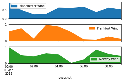
The wind generators have a per unit limit for each time step, given by the weather potentials at the site.
[9]:
network.generators_t.p_max_pu.plot.area(subplots=True)
plt.tight_layout()
Alright now we know how the network looks like, where the generators and lines are. Now, let’s perform a optimization of the operation and capacities.
[10]:
network.lopf();
INFO:pypsa.opf:Performed preliminary steps
INFO:pypsa.opf:Building pyomo model using `kirchhoff` formulation
INFO:pypsa.opf:Solving model using glpk
WARNING:pyomo.solvers:Could not locate the 'glpsol' executable, which is required for solver 'glpk'
---------------------------------------------------------------------------
ApplicationError                          Traceback (most recent call last)
/tmp/ipykernel_155/3801474310.py in <module>
----> 1 network.lopf();

~/checkouts/readthedocs.org/user_builds/pypsa-docs-staging/envs/latest/lib/python3.7/site-packages/pypsa/components.py in lopf(self, snapshots, pyomo, solver_name, solver_options, solver_logfile, formulation, keep_files, extra_functionality, multi_investment_periods, **kwargs)
    646
    647         if pyomo:
--> 648             return network_lopf(self, **args)
    649         else:
    650             return network_lopf_lowmem(self, **args)

~/checkouts/readthedocs.org/user_builds/pypsa-docs-staging/envs/latest/lib/python3.7/site-packages/pypsa/opf.py in network_lopf(network, snapshots, solver_name, solver_io, skip_pre, extra_functionality, multi_investment_periods, solver_logfile, solver_options, keep_files, formulation, ptdf_tolerance, free_memory, extra_postprocessing)
   1663                               solver_logfile=solver_logfile, solver_options=solver_options,
   1664                               keep_files=keep_files, free_memory=free_memory,
-> 1665                               extra_postprocessing=extra_postprocessing)

~/checkouts/readthedocs.org/user_builds/pypsa-docs-staging/envs/latest/lib/python3.7/site-packages/pypsa/opf.py in network_lopf_solve(network, snapshots, formulation, solver_options, solver_logfile, keep_files, free_memory, extra_postprocessing)
   1563             network.results = network.opt.solve(*args, suffixes=["dual"], keepfiles=keep_files, logfile=solver_logfile, options=solver_options)
   1564     else:
-> 1565         network.results = network.opt.solve(*args, suffixes=["dual"], keepfiles=keep_files, logfile=solver_logfile, options=solver_options)
   1566
   1567     if logger.isEnabledFor(logging.INFO):

~/checkouts/readthedocs.org/user_builds/pypsa-docs-staging/envs/latest/lib/python3.7/site-packages/pyomo/opt/base/solvers.py in solve(self, *args, **kwds)
    510         """ Solve the problem """
    511
--> 512         self.available(exception_flag=True)
    513         #
    514         # If the inputs are models, then validate that they have been

~/checkouts/readthedocs.org/user_builds/pypsa-docs-staging/envs/latest/lib/python3.7/site-packages/pyomo/opt/solver/shellcmd.py in available(self, exception_flag)
    123             if exception_flag:
    124                 msg = "No executable found for solver '%s'"
--> 125                 raise ApplicationError(msg % self.name)
    126             return False
    127         return True

ApplicationError: No executable found for solver 'glpk'
The objective is given by:
[11]:
network.objective
---------------------------------------------------------------------------
AttributeError                            Traceback (most recent call last)
/tmp/ipykernel_155/2252453118.py in <module>
----> 1 network.objective

AttributeError: 'Network' object has no attribute 'objective'
Why is this number negative? It considers the starting point of the optimization, thus the existent capacities given by network.generators.p_nom are taken into account.
The real system cost are given by
[12]:
network.objective + network.objective_constant
---------------------------------------------------------------------------
AttributeError                            Traceback (most recent call last)
/tmp/ipykernel_155/3503365564.py in <module>
----> 1 network.objective + network.objective_constant

AttributeError: 'Network' object has no attribute 'objective'
The optimal capacities are given by p_nom_opt for generators, links and storages and s_nom_opt for lines.
Let’s look how the optimal capacities for the generators look like.
[13]:
network.generators.p_nom_opt.div(1e3).plot.bar(ylabel='GW', figsize=(8,3))
plt.tight_layout()
Their production is again given as a time-series in network.generators_t.
[14]:
network.generators_t.p.div(1e3).plot.area(subplots=True, ylabel='GW')
plt.tight_layout()
---------------------------------------------------------------------------
TypeError                                 Traceback (most recent call last)
/tmp/ipykernel_155/3043318860.py in <module>
----> 1 network.generators_t.p.div(1e3).plot.area(subplots=True, ylabel='GW')
      2 plt.tight_layout()

~/checkouts/readthedocs.org/user_builds/pypsa-docs-staging/envs/latest/lib/python3.7/site-packages/pandas/plotting/_core.py in area(self, x, y, **kwargs)
   1494             >>> ax = df.plot.area(x='day')
   1495         """
-> 1496         return self(kind="area", x=x, y=y, **kwargs)
   1497
   1498     def pie(self, **kwargs):

~/checkouts/readthedocs.org/user_builds/pypsa-docs-staging/envs/latest/lib/python3.7/site-packages/pandas/plotting/_core.py in __call__(self, *args, **kwargs)
    970                     data.columns = label_name
    971
--> 972         return plot_backend.plot(data, kind=kind, **kwargs)
    973
    974     __call__.__doc__ = __doc__

~/checkouts/readthedocs.org/user_builds/pypsa-docs-staging/envs/latest/lib/python3.7/site-packages/pandas/plotting/_matplotlib/__init__.py in plot(data, kind, **kwargs)
     69             kwargs["ax"] = getattr(ax, "left_ax", ax)
     70     plot_obj = PLOT_CLASSES[kind](data, **kwargs)
---> 71     plot_obj.generate()
     72     plot_obj.draw()
     73     return plot_obj.result

~/checkouts/readthedocs.org/user_builds/pypsa-docs-staging/envs/latest/lib/python3.7/site-packages/pandas/plotting/_matplotlib/core.py in generate(self)
    284     def generate(self):
    285         self._args_adjust()
--> 286         self._compute_plot_data()
    287         self._setup_subplots()
    288         self._make_plot()

~/checkouts/readthedocs.org/user_builds/pypsa-docs-staging/envs/latest/lib/python3.7/site-packages/pandas/plotting/_matplotlib/core.py in _compute_plot_data(self)
    451         # no non-numeric frames or series allowed
    452         if is_empty:
--> 453             raise TypeError("no numeric data to plot")
    454
    455         self.data = numeric_data.apply(self._convert_to_ndarray)

TypeError: no numeric data to plot
What are the Locational Marginal Prices in the network. From the optimization these are given for each bus and snapshot.
[15]:
network.buses_t.marginal_price.mean(1).plot.area(figsize=(8,3), ylabel='Euro per MWh')
plt.tight_layout()
We can inspect futher quantities as the active power of AC-DC converters and HVDC link.
[16]:
network.links_t.p0
[16]:
| snapshot |
|---|
| 2015-01-01 00:00:00 |
| 2015-01-01 01:00:00 |
| 2015-01-01 02:00:00 |
| 2015-01-01 03:00:00 |
| 2015-01-01 04:00:00 |
| 2015-01-01 05:00:00 |
| 2015-01-01 06:00:00 |
| 2015-01-01 07:00:00 |
| 2015-01-01 08:00:00 |
| 2015-01-01 09:00:00 |
[17]:
network.lines_t.p0
[17]:
| snapshot |
|---|
| 2015-01-01 00:00:00 |
| 2015-01-01 01:00:00 |
| 2015-01-01 02:00:00 |
| 2015-01-01 03:00:00 |
| 2015-01-01 04:00:00 |
| 2015-01-01 05:00:00 |
| 2015-01-01 06:00:00 |
| 2015-01-01 07:00:00 |
| 2015-01-01 08:00:00 |
| 2015-01-01 09:00:00 |
…or the active power injection per bus.
[18]:
network.buses_t.p
[18]:
| snapshot |
|---|
| 2015-01-01 00:00:00 |
| 2015-01-01 01:00:00 |
| 2015-01-01 02:00:00 |
| 2015-01-01 03:00:00 |
| 2015-01-01 04:00:00 |
| 2015-01-01 05:00:00 |
| 2015-01-01 06:00:00 |
| 2015-01-01 07:00:00 |
| 2015-01-01 08:00:00 |
| 2015-01-01 09:00:00 |